2.1. Free Fermi gas (FFG)#
In this tutorial, you will learn how to use the free Fermi gas module to make predictions on thermodynamical properties.
Import the libraries that will be employed in this tutorial.
# Import numpy
import numpy as np
# Import matplotlib
import matplotlib.pyplot as plt
# Import nucleardatapy package
! pip install nucleardatapy --quiet
import nucleardatapy as nuda
%matplotlib inline
You can simply print out the properties of the nuda’s function that we will use:
# Explore the nucleardatapy module to find the correct attribute
print(dir(nuda.matter.setupFFGNuc))
['__class__', '__delattr__', '__dict__', '__dir__', '__doc__', '__eq__', '__format__', '__ge__', '__getattribute__', '__getstate__', '__gt__', '__hash__', '__init__', '__init_subclass__', '__le__', '__lt__', '__module__', '__ne__', '__new__', '__reduce__', '__reduce_ex__', '__repr__', '__setattr__', '__sizeof__', '__str__', '__subclasshook__', '__weakref__', 'print_outputs']
Then, define the density den and isospin parameter delta for which the FFG module will be evaluated.
The density goes from 0.01 to 0.3 with 10 points and the isospin parameter is zero (SM):
den = np.linspace(0.01,0.3,num=10)
delta = np.zeros( den.size )
Finaly instantiate the object ffg by calling the class setupFFGNuc:
ffg = nuda.matter.setupFFGNuc( den = den, delta = delta )
Print on screen the outputs:
ffg.print_outputs( )
- Print output:
   den: [0.01 0.04 0.07 0.11 0.14 0.17 0.2  0.24 0.27 0.3 ] in fm$^{-3}$
   delta: [0. 0. 0. 0. 0. 0. 0. 0. 0. 0.]
   kf_n: [0.53 0.86 1.03 1.16 1.27 1.36 1.44 1.52 1.58 1.64] in fm$^{-1}$
   e2a_int: [ 3.47  9.04 13.16 16.69 19.87 22.79 25.53 28.11 30.57 32.93] in MeV
   pre: [0.02 0.25 0.65 1.17 1.82 2.56 3.41 4.34 5.36 6.46] in MeV fm$^{-3}$
   cs2: [0.004 0.01  0.015 0.019 0.022 0.025 0.028 0.031 0.033 0.036] in c$^{2}$
The non-relativistic quantities are:
   e2a_int_nr: [ 3.48  9.1  13.27 16.87 20.12 23.12 25.94 28.61 31.16 33.62] in MeV
   pre_nr: [0.02 0.26 0.66 1.2  1.86 2.64 3.52 4.49 5.56 6.72] in MeV fm$^{-3}$
   cs2_nr: [0.004 0.011 0.015 0.019 0.023 0.026 0.029 0.032 0.035 0.038] in c$^{2}$
Now, we can also compute the FFG with a modified mass (constant) in the following way:
ffg = nuda.matter.setupFFGNuc( den = den, delta = delta, ms = 0.6 )
ffg.print_outputs( )
- Print output:
   den: [0.01 0.04 0.07 0.11 0.14 0.17 0.2  0.24 0.27 0.3 ] in fm$^{-3}$
   delta: [0. 0. 0. 0. 0. 0. 0. 0. 0. 0.]
   kf_n: [0.53 0.86 1.03 1.16 1.27 1.36 1.44 1.52 1.58 1.64] in fm$^{-1}$
   e2a_int: [ 5.77 14.92 21.63 27.33 32.42 37.09 41.43 45.51 49.38 53.08] in MeV
   pre: [ 0.04  0.41  1.05  1.89  2.91  4.08  5.39  6.84  8.41 10.09] in MeV fm$^{-3}$
   cs2: [0.011 0.027 0.039 0.048 0.055 0.062 0.068 0.073 0.078 0.083] in c$^{2}$
The non-relativistic quantities are:
   e2a_int_nr: [ 5.8  15.16 22.12 28.12 33.53 38.53 43.23 47.68 51.94 56.03] in MeV
   pre_nr: [ 0.04  0.43  1.1   2.    3.1   4.4   5.86  7.49  9.27 11.21] in MeV fm$^{-3}$
   cs2_nr: [0.011 0.029 0.041 0.051 0.06  0.068 0.076 0.082 0.089 0.095] in c$^{2}$
The complete outputs are available in the following way:
ffg.__dict__
{'label': 'FFG $\\,\\delta=$0.0',
 'note': '',
 'den': array([0.01      , 0.04222222, 0.07444444, 0.10666667, 0.13888889,
        0.17111111, 0.20333333, 0.23555556, 0.26777778, 0.3       ]),
 'delta': array([0., 0., 0., 0., 0., 0., 0., 0., 0., 0.]),
 'ms': 0.6,
 'x_n': array([0.5, 0.5, 0.5, 0.5, 0.5, 0.5, 0.5, 0.5, 0.5, 0.5]),
 'x_p': array([0.5, 0.5, 0.5, 0.5, 0.5, 0.5, 0.5, 0.5, 0.5, 0.5]),
 'den_n': array([0.005     , 0.02111111, 0.03722222, 0.05333333, 0.06944444,
        0.08555556, 0.10166667, 0.11777778, 0.13388889, 0.15      ]),
 'den_p': array([0.005     , 0.02111111, 0.03722222, 0.05333333, 0.06944444,
        0.08555556, 0.10166667, 0.11777778, 0.13388889, 0.15      ]),
 'kf_nuc': array([0.52900974, 0.85502215, 1.03293842, 1.16450112, 1.27160678,
        1.36319004, 1.44388696, 1.51645008, 1.58266323, 1.64375626]),
 'kf_n': array([0.52900974, 0.85502215, 1.03293842, 1.16450112, 1.27160678,
        1.36319004, 1.44388696, 1.51645008, 1.58266323, 1.64375626]),
 'kf_p': array([0.52900974, 0.85502215, 1.03293842, 1.16450112, 1.27160678,
        1.36319004, 1.44388696, 1.51645008, 1.58266323, 1.64375626]),
 'eF_n': array([573.32253289, 588.44538774, 599.45574082, 608.77268689,
        617.06070065, 624.62769737, 631.64869816, 638.23536908,
        644.46453039, 650.39192458]),
 'eF_n_int': array([ 9.58332529, 24.70618014, 35.71653322, 45.03347929, 53.32149305,
        60.88848977, 67.90949056, 74.49616148, 80.72532279, 86.65271698]),
 'eF_n_int_nr': array([ 9.67143798, 25.26494998, 36.87334867, 46.86445098, 55.88167136,
        64.2209204 , 72.04935624, 79.4730631 , 86.5646824 , 93.37670705]),
 'eF_p': array([572.55952168, 587.7020108 , 598.72603447, 608.05416161,
        616.35183738, 623.92743125, 630.95622434, 637.5500494 ,
        643.78584179, 649.71942768]),
 'eF_p_int': array([ 9.59631388, 24.738803  , 35.76282667, 45.09095381, 53.38862958,
        60.96422345, 67.99301654, 74.5868416 , 80.82263399, 86.75621988]),
 'eF_p_int_nr': array([ 9.67143798, 25.26494998, 36.87334867, 46.86445098, 55.88167136,
        64.2209204 , 72.04935624, 79.4730631 , 86.5646824 , 93.37670705]),
 'e2a_rm': array([563.3512077, 563.3512077, 563.3512077, 563.3512077, 563.3512077,
        563.3512077, 563.3512077, 563.3512077, 563.3512077, 563.3512077]),
 'eps_rm': array([  5.63351208,  23.78593988,  41.93836768,  60.09079549,
         78.24322329,  96.3956511 , 114.5480789 , 132.7005067 ,
        150.85293451, 169.00536231]),
 'eps': array([  5.69118961,  24.41607596,  43.54871519,  63.00632965,
         82.74662667, 102.7419156 , 122.97200004, 143.42119548,
        164.07680589, 184.92824645]),
 'e2a': array([569.11896085, 578.27548332, 584.9827413 , 590.68434047,
        595.77571202, 600.43976647, 604.78032808, 608.8635657 ,
        612.73495974, 616.42748818]),
 'e2a_int': array([ 5.76775315, 14.92427562, 21.6315336 , 27.33313277, 32.42450432,
        37.08855877, 41.42912038, 45.512358  , 49.38375204, 53.07628048]),
 'e2a_int_nr': array([ 5.80286279, 15.15896999, 22.1240092 , 28.11867059, 33.52900282,
        38.53255224, 43.22961374, 47.68383786, 51.93880944, 56.02602423]),
 'e2a_nr': array([569.15407049, 578.51017769, 585.4752169 , 591.46987829,
        596.88021052, 601.88375994, 606.58082144, 611.03504556,
        615.29001714, 619.37723193]),
 'eps_int': array([ 0.05767753,  0.63013608,  1.6103475 ,  2.91553416,  4.50340338,
         6.3462645 ,  8.42392114, 10.72068877, 13.22387138, 15.92288414]),
 'eps_int_nr': array([ 0.05802863,  0.6400454 ,  1.64700957,  2.99932486,  4.65680595,
         6.59334783,  8.79002146, 11.23219292, 13.90805897, 16.80780727]),
 'eps_nr': array([  5.6915407 ,  24.42598528,  43.58537726,  63.09012035,
         82.90002924, 102.98899892, 123.33810036, 143.93269962,
        164.76099348, 185.81316958]),
 'esym_nr': array([ 3.40860771,  8.90439492, 12.99566628, 16.51693668, 19.69497153,
        22.63406172, 25.39312059, 28.00953652, 30.5089113 , 32.90974557]),
 'esym2_nr': array([ 3.22381266,  8.42164999, 12.29111622, 15.62148366, 18.62722379,
        21.40697347, 24.01645208, 26.49102103, 28.85489413, 31.12556902]),
 'esym4_nr': array([0.11940047, 0.31191296, 0.45522653, 0.57857347, 0.68989718,
        0.79285087, 0.88949823, 0.98114893, 1.06869978, 1.15279885]),
 'pre': array([ 0.03822066,  0.41370245,  1.05027312,  1.89110227,  2.90702181,
         4.07891207,  5.39283374,  6.83797603,  8.40560506, 10.08845639]),
 'pre_nr': array([ 0.03868575,  0.42669693,  1.09800638,  1.99954991,  3.1045373 ,
         4.39556522,  5.86001431,  7.48812861,  9.27203932, 11.20520485]),
 'h2a': array([572.94102729, 588.07369927, 599.09088764, 608.41342425,
        616.70626901, 624.27756431, 631.30246125, 637.89270924,
        644.12518609, 650.05567613]),
 'h2a_nr': array([573.02264568, 588.61615768, 600.22455637, 610.21565868,
        619.23287906, 627.5721281 , 635.40056394, 642.8242708 ,
        649.9158901 , 656.72791475]),
 'cs2': array([0.0110652 , 0.02743741, 0.03858471, 0.0475482 , 0.05518242,
        0.06188839, 0.06789585, 0.07335214, 0.07835889, 0.08298996]),
 'cs2_nr': array([0.01125196, 0.02861508, 0.04095506, 0.05119988, 0.06016226,
        0.06822156, 0.07559468, 0.08242072, 0.08879578, 0.09478985]),
 'den_unit': 'fm$^{-3}$',
 'kf_unit': 'fm$^{-1}$',
 'e2a_unit': 'MeV',
 'eps_unit': 'MeV fm$^{-3}$',
 'pre_unit': 'MeV fm$^{-3}$',
 'cs2_unit': 'c$^{2}$'}
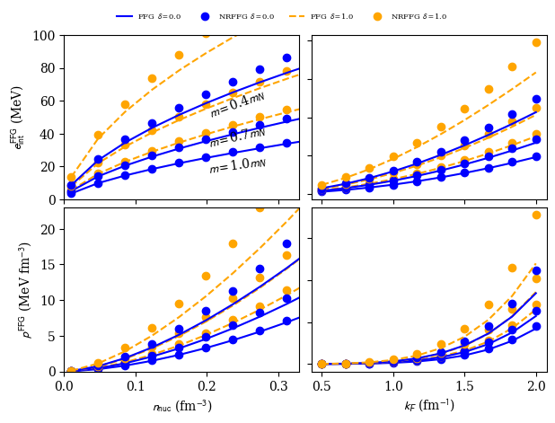
plot:
den = np.linspace(0.01,0.35,10)
kfn = np.linspace(0.5,2.0,10)
mss = [ 1.0, 0.7, 0.4 ]
nuda.fig.matter_setupFFGNuc_EP_fig( pname=None, den = den, kf = kfn, mss = mss )
Plot name: None
plot $\delta=0$ (SM)
plot $\delta=1$ (NM)
plot $\delta=0$ (SM)
plot $\delta=1$ (NM)
plot $\delta=0$ (SM)
plot $\delta=1$ (NM)